Physics–Informed Source Separation

Source Separation: From Smoothies to PDEs

Physical systems are often measured as mixtures of signals. For instance, seismometers measure not only the magnitude of earthquakes but also any other vibrations significant enough to register, such as mining explosions. Such extraneous signals can corrupt measurements (e.g., pressure waves from mining explosions mixed with seismic pressure waves from earthquakes), so it is often vital to isolate the signals of interest. This process is called source separation and is a type of inverse problem since the goal is to infer the original source signals (i.e., causes) from a collection of observed mixtures (i.e., effects). Source separation problems are often blind due to the absence of a well–defined model for how the constituent signals were mixed or of the sources themselves.

As an analogy for blind source separation, imagine if I concocted a delicious smoothie and tasked you with reverse engineering the recipe! With training, you can become better at deconstructing the smoothie by incorporating knowledge of how smoothies are typically made, how Justin likes to make smoothies, which ingredients are reasonable for smoothies, etc. This accumulated knowledge of “smoothie deconstruction” can be thought of in a statistical sense as a priori information. One could take this analogy further by assuming that this a priori information represents a Bayesian prior that updates over time with each taste test! Training a machine learning model with this a priori information would be an instance of “smoothie–informed machine learning.”

Fortunately, unlike smoothies, many physical systems yield observed signals whose constituent mixed sources abide by known partial differential equations (PDEs), such as the linear advection equation. This information can be leveraged as a priori information, yielding physics–informed source separation algorithms with improved efficiency, accuracy, and mathematical well–posedness.

This post elaborates on these points by explaining:

• An example blind source separation (BSS) problem from physics
• How to regularize the aforementioned BSS problem with physically meaningful loss terms that incorporate a priori information about the constituent source signals
• The penalty method for converting numerical constrained optimization problems into unconstrained ones
• The method of multipliers for improving convergence of the penalty method
• The Gauss–Newton algorithm and Levenberg–Marquardt algorithm for solving nonlinear least–squares problems
• Implementation in Python using NumPy, JAX, and JAXopt libraries for high–performance computing–based numerical simulation of PDEs and optimization.

The Linear Advection PDE

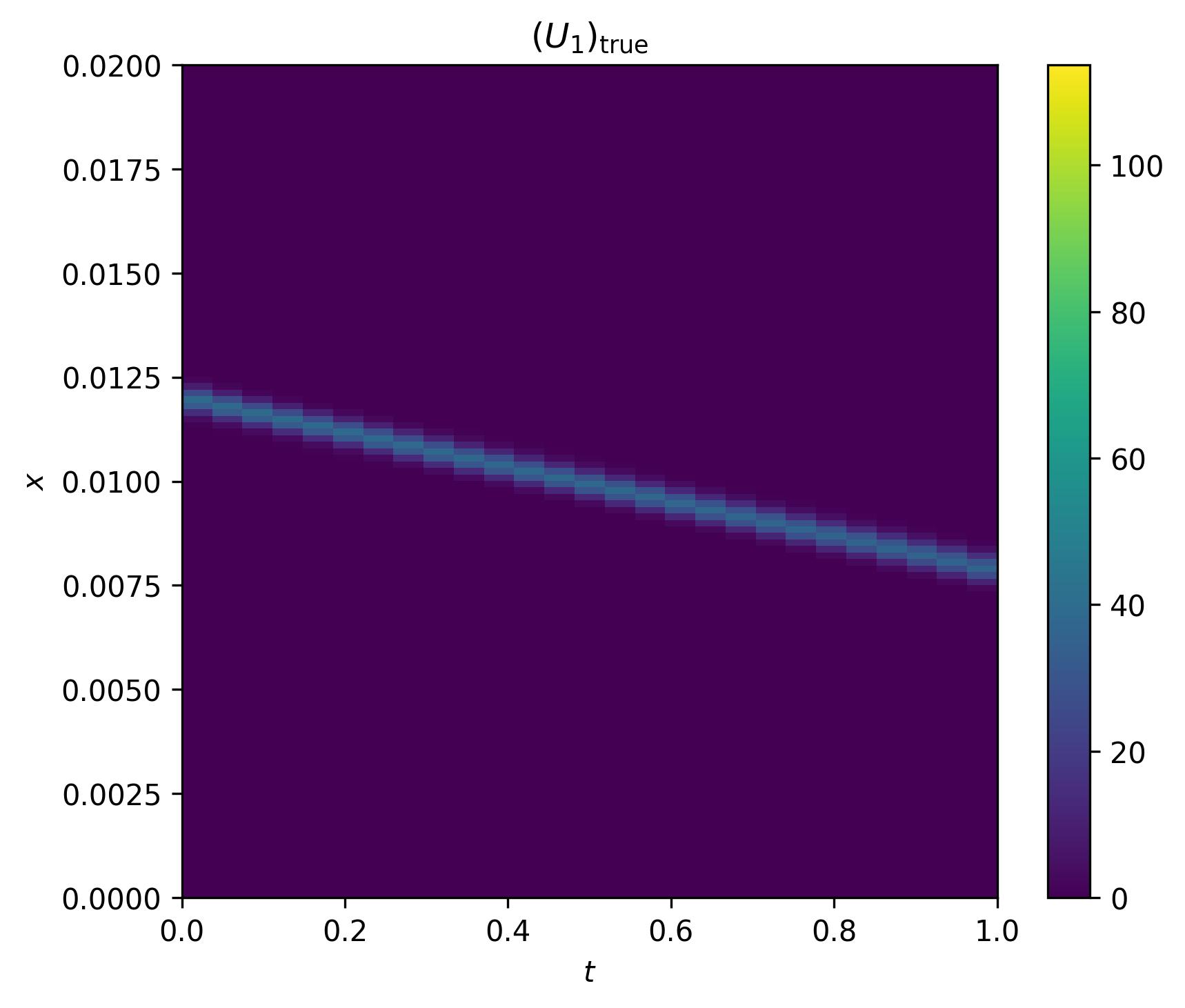
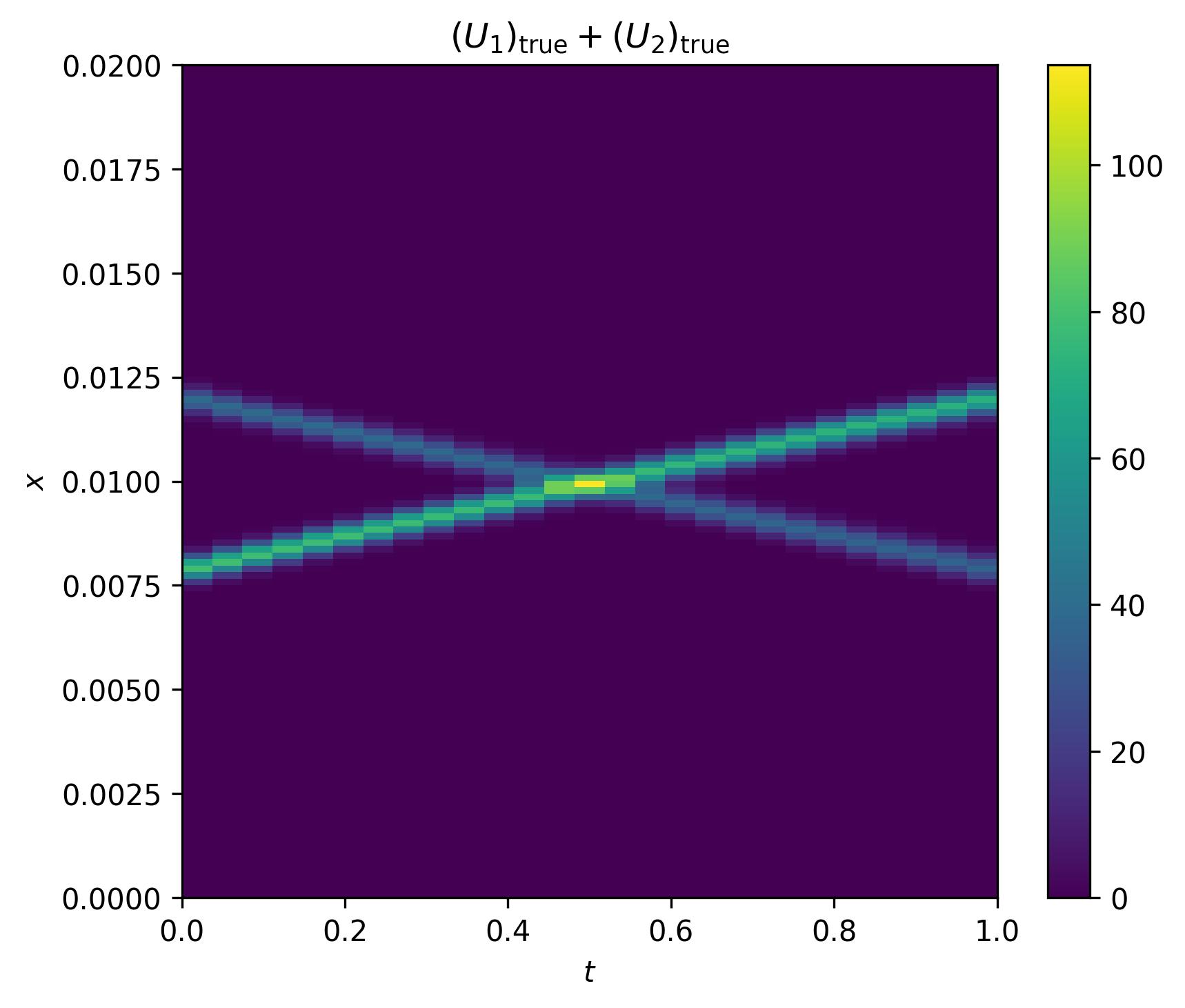
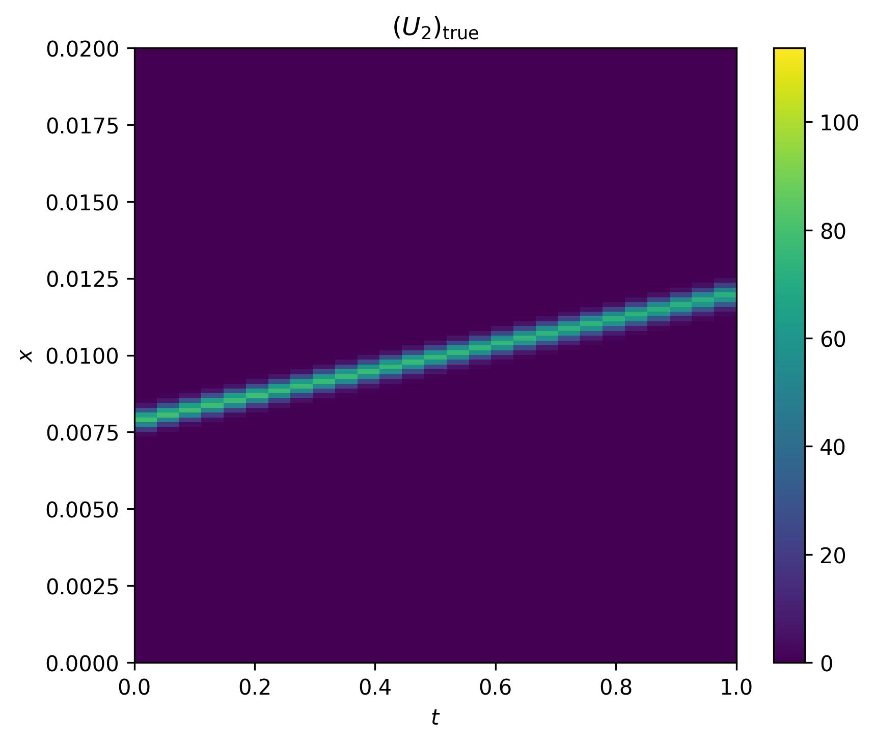
Physics is often expressed in the language of partial differential equations (PDEs). These equations leverage partial derivatives to model how multivariate dependent variables respond to changes in their independent variables, often space and time. For instance, the linear advection equation models how the value of an advected quantity changes according to the spatial gradient of that quantity and the underlying velocity field. The algebraic structure of this PDE and the spectral properties of the differential operators composing it conspire together to model translational motion called advection.

This post uses JAX for physics–informed source separation with simulated data from a 1–dimensional linear advection PDE. This equation is linear, ubiquitous, and well–suited to modeling the transport of localized signals that are easily distinguished by the naked eye but not necessarily to a blind source separation algorithm. Linearity of the advection equation is particularly helpful here since it allows us to easily model the (trivially) coupled evolution of multiple advecting signals by virtue of the principle of superposition:

where $u = \sum_{i=1}^{n}u_i$ is the observed signal and $f = \sum_{i=1}^{n}c_i u_i$ is the total flux.

The rest of this post will assume that there are only two advecting pulses, yielding the following model of the observed flow field:

where $c_i$ are constants quantifying advection speed. In general, determining the optimal value of $n$ (i.e., the number of sources being mixed) may not be trivial. However, there are plenty of data–driven methods to accomplish this. For instance, one could apply the line Hough transform to the Minkowski spacetime diagram of the observed solution then compute the number of disjoint maxima in this Hough space.

Constrained Optimization for Physics–Informed Source Separation

Recall that our observed signal is the superposition of multiple individually advecting signals. As such, we can pose the following BSS problem:

where $U_1\in\mathbb{R}^{n\times K}$ is a matrix whose $j$th column is source one at timestamp $j$, $u_1(:, t_j)$; $U_2\in\mathbb{R}^{n\times K}$ is a matrix whose $j$th column is source two at timestamp $j$, $u_2(:, t_j)$; and $U\in\mathbb{R}^{n\times K}$ is a matrix whose $j$th column is the observed signal at timestamp $j$, $u(:, t_j)$. The $1/2$ in front of the Frobenius norm is a fudge factor used to remove irrelevant coefficients of $2$ from gradients of the norm with respect to design variables $U_1$, $U_2$, or $W=[U_1^\top \quad U_2^\top]^\top$ where $U_1 + U_2 - U = [I \quad I]~W - U$. Neglecting this $1/2$ does not change the optimal $(\hat{U}_1,\hat{U}_2)$.

This BSS problem is unfortunately ill–posed since there are many equivalently–optimal solutions, most of which are physically meaningless. For instance, both $(\hat{U}_1,\hat{U}_2)=(U,0)$ and $(\hat{U}_1,\hat{U}_2)=(0,U)$ are valid solutions even though we assume $U_1\neq0\neq U_2$ by formulation of the residual in the norm being minimized. This ill–posedness is a common obstacle in the solution of computational inverse problems, such as source separation. Fortunately, a priori knowledge of signals $U_1$ and $U_2$ can be leveraged to regularize this problem, making it well–posed. One such regularization enforces that $\hat{U}_1$ and $\hat{U}_2$ are non–negative matrices:

Additionally, we can assume that $U_1$ and $U_2$ satisfy their own advection equations:

where $\dot{U}_i$ is a finite–difference–computed time derivative of $U_i$ and $U^\prime_i$ is a finite–difference–computed spatial derivative. Constants $c_i$ can be computed from observed snapshots $U$, such as from the slope of the $i$th line detected in Hough space via the line Hough transform of $U$.

Unconstrained Optimization for Physics–Informed Source Separation

Our constrained optimization problem can be converted into an unconstrained one through the penalty method. Doing so enables the solution of our constrained optimization problem by using optimizers for unconstrained problems:

where $\min$ is a function that computes the elementwise minimum of a matrix with the zero matrix of the same shape, thus penalizing negative values. Index $k$ is used to convey the $k$th iteration of the penalty method. In practice, one often starts the optimization procedure using a small value of $\mu^{(k)}$; obtains $(\hat{U}_1^{(k)}, \hat{U}_2^{(k)})$; then recursively solves for $(\hat{U}_1^{(k+1)}, \hat{U}_2^{(k+1)})$ until convergence using $\mu^{(k+1)} > \mu^{(k)}$, where $(\hat{U}_1^{(k)}, \hat{U}_2^{(k)})$ is the initial guess of $(\hat{U}_1^{(k+1)}, \hat{U}_2^{(k+1)})$.

Furthermore, we can express this least–squares problem’s objective function to be minimized using a single norm:

where $r^{(k)}$ is a single residual formed by stacking all constituent residuals in our objective function into a column vector. This notation with $r^{(k)}$ will facilitate the later use of the Levenberg–Marquardt algorithm for numerical optimization.

Augmenting the Penalty Method With Lagrange Multipliers

Recall that we previously converted a constrained optimization problem into an unconstrained one using the penalty method. Intuitively, one recovers the constrained optimization solution in the limit as the penalty term, $\mu^{(k)}$, introduced by the penalty method, goes to infinity. Unfortunately, naively increasing $\mu^{(k)}$ towards infinity can make this optimization problem ill–posed if $\mu^{(k)}$ gets too large. However, one can circumvent the need to increase $\mu^{(k)}$ towards infinity by leveraging the method of multipliers (aka, the augmented Lagrangian method). The method of multipliers is analogous to the method of Lagrange multipliers from analytical optimization theory and forms the foundation of a standard tool in numerical optimization called the alternating direction method of multipliers, which is not covered in this post.

The following equation represents the penalty method objective augmented with Lagrange multipliers:

with matrix–matrix inner product

In the method of multipliers, Lagrange multipliers are treated as dual variables that are updated each iteration:

where $[\cdot]_+ = \max(0,\cdot)$ clips negative entries to zero, ensuring that all Lagrange multipliers are positive (each element of $\Lambda_i^{(k)}$ is a Lagrange multiplier).

The Levenberg–Marquardt Algorithm for Least–Squares Problems

The Levenberg–Marquardt algorithm is a workhorse tool for solving both linear and nonlinear least–squares problems with objective function $\frac{1}{2} \left\lVert r \right\rVert_\text{F}^2$. This algorithm can be thought of as an extension of the Gauss–Newton algorithm that incorporates a trust region for regularization. Let’s derive this algorithm with calculus.

First, consider the optimization problem of identifying the parameter, $\hat{\beta}$, which minimizes the least–squares error of fitting observed data, $y$, with a curve, $f(x, \beta)$:

where the loss function, $\mathcal{L}$, for this problem is the norm being minimized above:

Let’s begin by linearizing function $f$ about $\beta$:

where $J=\frac{\partial f(x,\beta)}{\partial\beta}$ is the Jacobian of $f$.

This linearized $f$ is then plugged into the original residual to define a new loss function in terms of observed data, $y$; fit curve, $f$; Jacobian, $J$; and optimization parameter step, $\delta\beta$:

We want to compute the optimization step $\delta\beta$ that yields the minimal loss relative to our current position in the loss landscape, so let’s compute the gradient of this loss function with respect to $\delta\beta$:

Finally, setting this derivative equal to zero yields a system of linear equations used to compute the optimal step of optimization parameter $\beta$:

where the $\overset{!}{=}$ form of the familiar $=$ symbol conveys that we are coercing the expression to equal $0$. Application of this equation is known as the Gauss–Newton algorithm.

Solving the system of linear equations in the Gauss–Newton algorithm may, however, be ill–posed due to an ill–conditioned $J^\top J$. This conditioning can be improved through the following regularization:

yielding a system of linear equations whose application is known as the Levenberg–Marquardt algorithm.

There are various benefits to adding $\gamma I$ to $J^\top J$, namely those stemming from increasing the positive–definiteness of the system matrix. To convey these benefits, let’s first use the Rayleigh–Ritz quotient to show that eigenvalues of $J^\top J + \gamma I$ are larger than those of $J^\top J$ when $\gamma > 0$:

where $\lambda_i^{\text{LM}}$ is the $i$th largest eigenvalue of $J^\top J + \gamma I$, $\lambda_i^{\text{GN}}$ is the $i$th largest eigenvalue of $J^\top J$, and $\gamma \geq 0$. Thus, adding a sufficiently large value of $\gamma$ will make the system matrix in the Levenberg–Marquardt algorithm symmetric positive–definite. Importantly, if $J^\top J + \gamma I$ is symmetric positive–definite (meaning that it’s symmetric and all eigenvalues are positive), then:

• there exists a unique solution for $\delta\beta$
• the step taken is always a descent direction
• conjugate gradient, a fast and numerically stable solver, can be used.

Appropriately choosing $\gamma$ can significantly reduce the condition number of the system matrix at hand. As a simple example, let’s assume that $J^\top J$ is a symmetric positive–definite matrix such that its singular values are its eigenvalues, yielding a condition number $\kappa(J^\top J) = \lambda_1^{\text{GN}} / \lambda_n^{\text{GN}}$. Let’s assert that $\lambda_1^{\text{GN}}=100$ and $\lambda_n^{\text{GN}}=0.0001$ such that $\kappa(J^\top J) = 100 / 0.0001 = 1,000,000$—a very ill–conditioned system! Despite this enormous condition number, the condition number of $J^\top J + \gamma I$ with $\gamma=1$ is orders of magnitude smaller: $\kappa(J^\top J + 1I) = (\lambda_1^{\text{GN}} + 1) / (\lambda_n^{\text{GN}}+1) = (100 + 1) / (0.0001 + 1) = 100.99$. Notably, the Levenberg–Marquardt algorithm interpolates between Gauss–Newton and gradient descent: $\gamma=0$ yields Gauss–Newton; $\gamma\gg 0$ yields gradient descent.

Finally, the solution can be made scale invariant by regularizing with a diagonal matrix formed directly from $J^TJ$ instead of with an arbitrarily chosen identity matrix:

A diagonal matrix (rather than one with arbitrarily located nonzero elements) is added for regularization to preserve symmetry.

JAX for Physics–Informed Source Separation

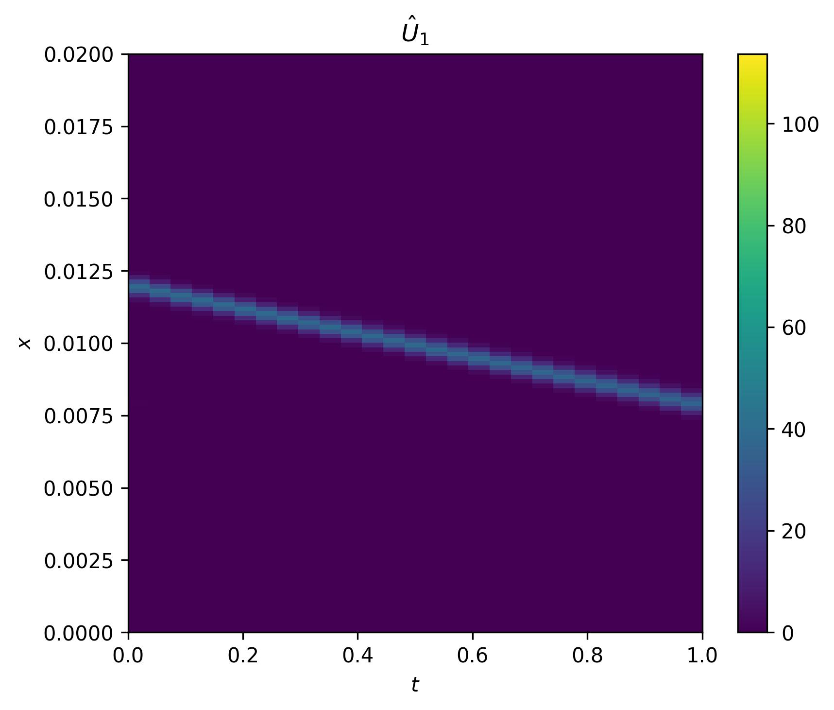
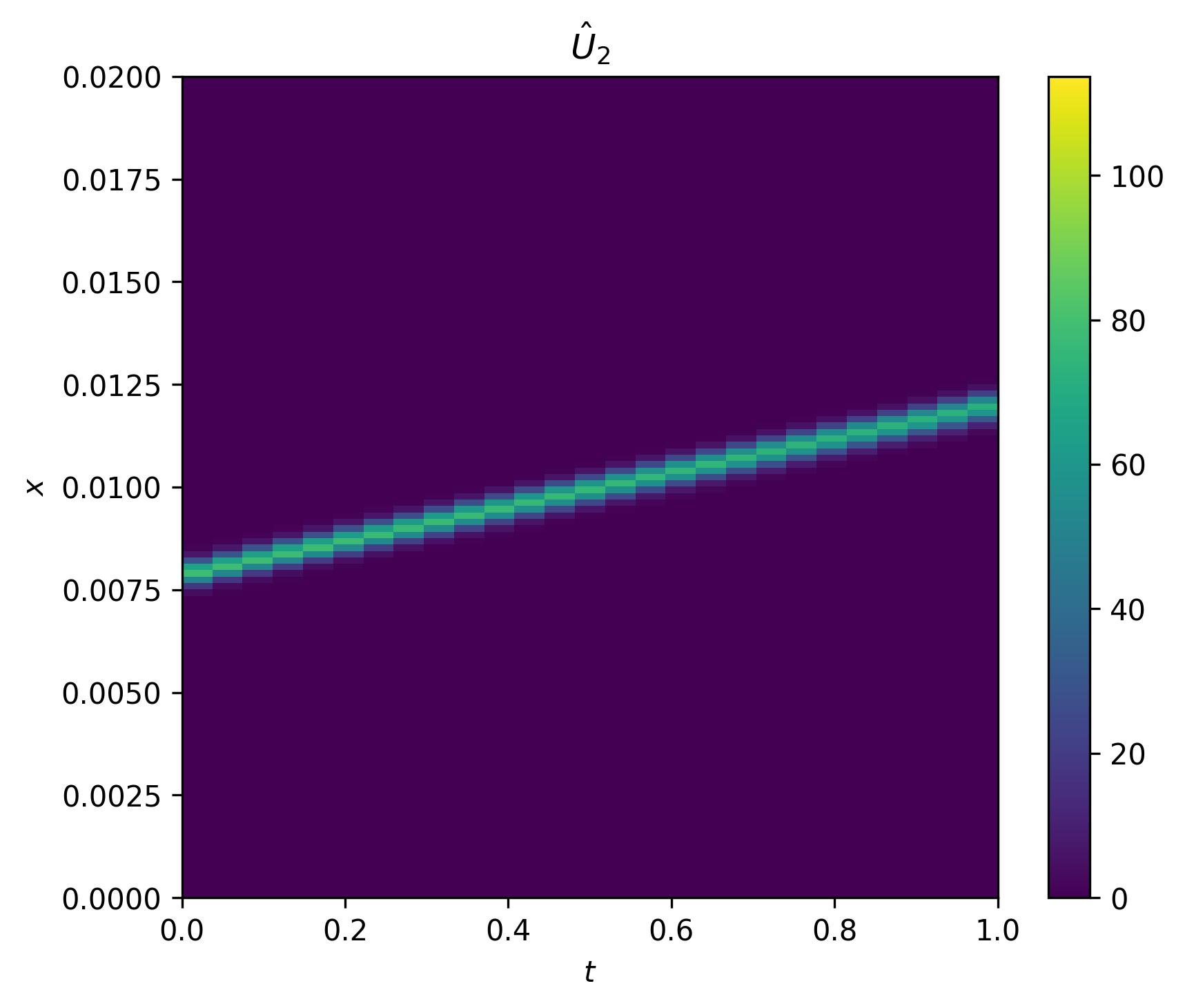
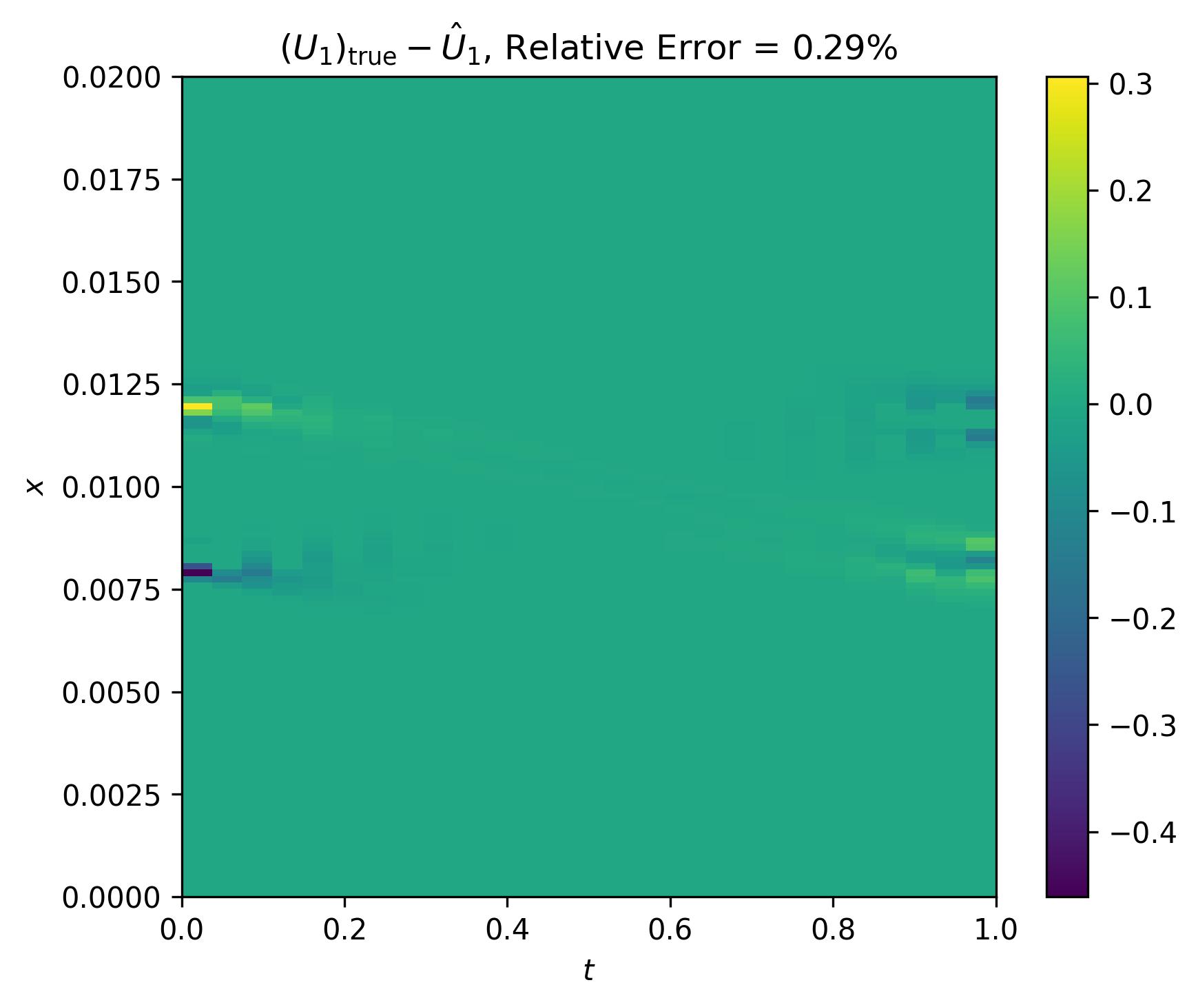
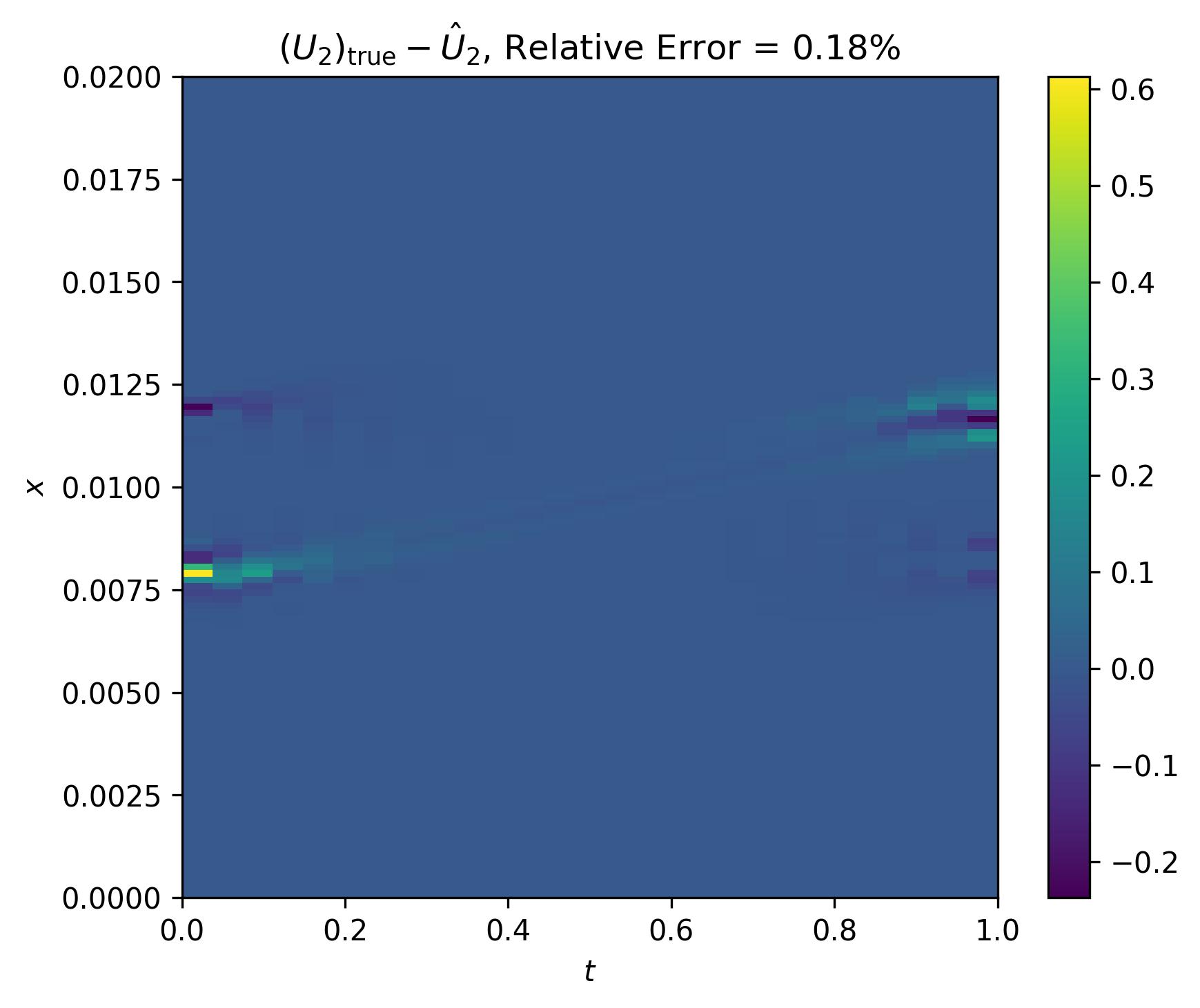
JAX is an incredible Python library that facilitates the use of automatic differentiation to easily compute Jacobians for numerical optimization (and anywhere else they may be used, such as in the numerical solution of nonlinear systems of ordinary differential equations using Newton’s method). One can also use it for just–in–time (JIT) compilation but we do not do so here. This library forms the backbone of another called JAXopt, which has an intuitive interface for calling a routine that uses the Levenberg–Marquardt algorithm to solve a least–squares problem, such as the one we posed using physics–informed regularization. The following illustrates how to solve the optimization problem we’ve discussed so far through JAXopt.

First, imports:

import numpy as np
import matplotlib.pyplot as plt
import jax
import jax.numpy as jnp
import jaxopt

Next, define helper functions for finite–difference simulation of the superposition of advecting signals:

# helper functions
def get_fwd_diff_op(u, dx):
    n = u.shape[0]
    main_diag = -1 * np.ones(n)
    super_diag = np.ones(n - 1)
    K = np.diag(main_diag) + np.diag(super_diag, k=1)
    K[-1, 0] = 1
    return K * (1 / dx)

def get_bwd_diff_op(u, dx):
    n = u.shape[0]
    main_diag = np.ones(n)
    sub_diag = -1 * np.ones(n - 1)
    K = np.diag(main_diag) + np.diag(sub_diag, k=-1)
    K[0, 0] = 1
    K[0, -1] = -1
    return K * (1 / dx)

def get_u_next(u_curr, a, dt, Kfwd, Kbwd):
    D = Kbwd if a >= 0.0 else Kfwd
    return u_curr - (a * dt) * (D @ u_curr)

def get_u0(x, mu):
    return np.exp(-((x - mu) ** 2) / 0.0002) / np.sqrt(0.0002 * np.pi)

Then, simulate the individual advection of two Gaussian pulses traveling towards and through each other:

# space
x0, xf = 0.0, 1.0
n = 2**7
x = np.linspace(x0, xf, num=n, endpoint=False)
dx = x[1] - x[0]

# speed
c1 = 10.0
c2 = -c1

# time
t0, tf = 0.0, 0.02
courant_number = 0.99
dt = courant_number * dx / max(abs(c1), abs(c2))
N_steps = int(np.ceil((tf - t0) / dt))
dt = (tf - t0) / N_steps
ts = np.linspace(t0, tf, N_steps + 1, endpoint=True)

# snapshots
U1 = np.zeros((n, N_steps + 1))
U2 = np.zeros((n, N_steps + 1))

mu1 = 0.4
mu2 = 1.0 - mu1
u1_curr = get_u0(x, mu1)
u2_curr = 2*get_u0(x, mu2)
U1[:, 0] = u1_curr
U2[:, 0] = u2_curr

# FD operators
Kfwd = get_fwd_diff_op(u1_curr, dx)
Kbwd = get_bwd_diff_op(u1_curr, dx)

# simulate
for j in range(1, N_steps + 1):
    u1_curr = get_u_next(u1_curr, c1, dt, Kfwd, Kbwd)
    U1[:, j] = u1_curr

    u2_curr = get_u_next(u2_curr, c2, dt, Kfwd, Kbwd)
    U2[:, j] = u2_curr

    if j % 100 == 0:
        print(f" Step {j:4d}/{N_steps:4d}, t = {ts[j]:.5f}")

# compute superposition solution
U = U1 + U2

Next, visualize the individual PDE solutions and their superposition (which will serve as our observed data that we wish to decompose via physics–informed source separation):

vmin = U.min()
vmax = U.max()

fig1, ax1 = plt.subplots(figsize=(6, 5))
im0 = ax1.imshow(U1, extent=(x0, xf, 0, tf), aspect='auto',
                 vmin=vmin, vmax=vmax)
ax1.set_xlabel(r'$t$')
ax1.set_ylabel(r'$x$')
ax1.set_title(r'$(U_1)_{\text{true}}$')
plt.colorbar(im0, ax=ax1)
fig1.tight_layout()
fig1.savefig("U1_true.jpg", dpi=300, bbox_inches='tight')
plt.close(fig1)

fig2, ax2 = plt.subplots(figsize=(6, 5))
im1 = ax2.imshow(U2, extent=(x0, xf, 0, tf), aspect='auto',
                 vmin=vmin, vmax=vmax)
ax2.set_xlabel(r'$t$')
ax2.set_ylabel(r'$x$')
ax2.set_title(r'$(U_2)_{\text{true}}$')
plt.colorbar(im1, ax=ax2)
fig2.tight_layout()
fig2.savefig("U2_true.jpg", dpi=300, bbox_inches='tight')
plt.close(fig2)

fig3, ax3 = plt.subplots(figsize=(6, 5))
im2 = ax3.imshow(U, extent=(x0, xf, 0, tf), aspect='auto',
                 vmin=vmin, vmax=vmax)
ax3.set_xlabel(r'$t$')
ax3.set_ylabel(r'$x$')
ax3.set_title(r'$(U_1)_{\text{true}} + (U_2)_{\text{true}}$')
plt.colorbar(im2, ax=ax3)
fig3.tight_layout()
fig3.savefig("U_sum_true.jpg", dpi=300, bbox_inches='tight')
plt.close(fig3)

After that, define helper functions for computing the residual that will be minimized:

def dUdt_center(U, dt):
    return (U[:, 2:] - U[:, :-2]) / (2 * dt)

def dUdx_center(U, dx):
    return (U[2:, :] - U[:-2, :]) / (2 * dx)

def pde_res(U, c, dt, dx):
    dt_term = dUdt_center(U, dt)[1:-1, :]
    dx_term = dUdx_center(U, dx)[:, 1:-1]
    return dt_term + c * dx_term

def get_residual(U_obs, dx, dt, c1, c2, reg_pde1, reg_pde2, mu, lam_1, lam_2, x):
    nx, nt = U_obs.shape
    U12 = x.reshape((2 * nx, nt))
    U1, U2 = U12[:nx, :], U12[nx:, :]

    r_dec = U1 + U2 - U_obs
    r_pde1 = jnp.sqrt(2.0 * reg_pde1) * pde_res(U1, c1, dt, dx)
    r_pde2 = jnp.sqrt(2.0 * reg_pde2) * pde_res(U2, c2, dt, dx)

    viol1 = -jnp.minimum(U1, 0.0)
    viol2 = -jnp.minimum(U2, 0.0)

    r_pen1 = jnp.sqrt(mu) * viol1
    r_pen2 = jnp.sqrt(mu) * viol2

    r_mm1 = jnp.sum(lam_1 * viol1)
    r_mm2 = jnp.sum(lam_2 * viol2)

    return jnp.concatenate([
        r_dec.ravel(),
        r_pde1.ravel(),
        r_pde2.ravel(),
        r_pen1.ravel(),
        r_pen2.ravel(),
        jnp.atleast_1d(r_mm1),
        jnp.atleast_1d(r_mm2),
    ])

Now pose the physics–informed source separation problem with JAX’s jax.numpy syntax. With residuals defined in this way, the Levenberg–Marquardt algorithm can be implemented to compute optimal $U_1$ and $U_2$ through the jaxopt.LevenbergMarquardt method:

nx, nt = U.shape
x = jnp.concatenate([U, U], axis=0).ravel()

lam_pde1 = 1e-6
lam_pde2 = 1e-6

mu = 1e3
mu_max = 1e6
outer_iters = 2
lm_maxiter = 50

lam_1 = jnp.zeros_like(U)
lam_2 = jnp.zeros_like(U)

U1ks, U2ks = [], []
U1_iters, U2_iters = [], []

prev_viol = jnp.inf

for k in range(outer_iters):
    print("outer iter", k)

    solver = jaxopt.LevenbergMarquardt(
        residual_fun=lambda x_: get_residual(
            U, dx, dt, c1, c2,
            lam_pde1, lam_pde2,
            mu, lam_1, lam_2,
            x_
        ),
        maxiter=lm_maxiter
    )

    x = solver.run(init_params=x).params

    U12 = x.reshape((2 * nx, nt))
    U1_k, U2_k = U12[:nx, :], U12[nx:, :]
    U1ks.append(U1_k)
    U2ks.append(U2_k)

    viol1 = -jnp.minimum(U1_k, 0.0)
    viol2 = -jnp.minimum(U2_k, 0.0)

    lam_1 = jnp.maximum(0.0, lam_1 + mu * viol1)
    lam_2 = jnp.maximum(0.0, lam_2 + mu * viol2)

    viol = jnp.sqrt(jnp.linalg.norm(viol1, 'fro')**2 +
                    jnp.linalg.norm(viol2, 'fro')**2)
    if float(viol) < 0.8 * float(prev_viol):
        mu = min(mu_max, 2.0 * mu)
    prev_viol = viol

U_hat = np.array(x.reshape((2 * nx, nt)))
U1_hat, U2_hat = U_hat[:nx, :], U_hat[nx:, :]

Last but not least, visualize the sources inferred through our solved physics–informed source separation problem:

rel_err = np.linalg.norm(U1 - U1ks[0], ord='fro') / np.linalg.norm(U1, ord='fro')
perc_err = 100 * rel_err

fig_recon, ax_recon = plt.subplots(figsize=(6, 5))
im0 = ax_recon.imshow(U1ks[0], extent=(x0, xf, 0, tf), aspect='auto', vmin=vmin, vmax=vmax)
ax_recon.set_xlabel(r'$t$')
ax_recon.set_ylabel(r'$x$')
ax_recon.set_title(r'$\hat{U}_1$')
plt.colorbar(im0, ax=ax_recon)
fig_recon.tight_layout()
fig_recon.savefig("U1_reconstruction.jpg", dpi=300, bbox_inches='tight')
plt.close(fig_recon)

fig_err, ax_err = plt.subplots(figsize=(6, 5))
err = U1 - U1ks[0]
im1 = ax_err.imshow(err, extent=(x0, xf, 0, tf), aspect='auto')
ax_err.set_xlabel(r'$t$')
ax_err.set_ylabel(r'$x$')
ax_err.set_title(r'$(U_1)_{\text{true}} - \hat{U}_1$, ' + rf'Relative Error = {perc_err:.2f}%')
plt.colorbar(im1, ax=ax_err)
fig_err.tight_layout()
fig_err.savefig("U1_error.jpg", dpi=300, bbox_inches='tight')
plt.close(fig_err)

rel_err = np.linalg.norm(U2 - U2ks[0], ord='fro') / np.linalg.norm(U2, ord='fro')
perc_err = 100 * rel_err

fig_recon, ax_recon = plt.subplots(figsize=(6, 5))
im0 = ax_recon.imshow(U2ks[0], extent=(x0, xf, 0, tf), aspect='auto', vmin=vmin, vmax=vmax)
ax_recon.set_xlabel(r'$t$')
ax_recon.set_ylabel(r'$x$')
ax_recon.set_title(r'$\hat{U}_2$')
plt.colorbar(im0, ax=ax_recon)
fig_recon.tight_layout()
fig_recon.savefig("U2_reconstruction.jpg", dpi=300, bbox_inches='tight')
plt.close(fig_recon)

fig_err, ax_err = plt.subplots(figsize=(6, 5))
err = U2 - U2ks[0]
im1 = ax_err.imshow(err, extent=(x0, xf, 0, tf), aspect='auto')
ax_err.set_xlabel(r'$t$')
ax_err.set_ylabel(r'$x$')
ax_err.set_title(r'$(U_2)_{\text{true}} - \hat{U}_2$, ' + rf'Relative Error = {perc_err:.2f}%')
plt.colorbar(im1, ax=ax_err)
fig_err.tight_layout()
fig_err.savefig("U2_error.jpg", dpi=300, bbox_inches='tight')
plt.close(fig_err)

Conclusion

In this post we demonstrated how to use JAX and JAXopt to implement the Levenberg–Marquardt algorithm for solving a least–squares problem whose objective function is formulated using the method of multipliers (aka, augmented Lagrangian method). This was applied to physics–informed source separation of the superposition of two advecting signals, with physics prescribed by 1D linear advection.